构造数据集

>>> from sklearn.datasets import load_iris
>>> import numpy as np
>>> iris = load_iris()
>>> iris.data
array([[ 5.1,  3.5,  1.4,  0.2],
       [ 4.9,  3. ,  1.4,  0.2],
       ....
       [ 5.9,  3. ,  5.1,  1.8]])
>>> iris.target
array([0, 0, 0, 0, 0, 0, ... , 2, 2, 2, 2, 2, 2, 2, 2, 2, 2,
       2, 2, 2, 2, 2, 2, 2, 2, 2, 2, 2, 2])
>>> iris.data.shape  
(150, 4)                   # 150个样本，每个样本4个特征
>>> iris.target.shape      # 每个样本的类别
(150,)
>>> # 下面开始构造训练集/测试集，120/30
>>> # 训练集
>>> train_data = np.concatenate((iris.data[0:40, :], iris.data[50:90, :], iris.data[100:140, :]), axis = 0)
>>> # 训练集样本类别
>>> train_target = np.concatenate((iris.target[0:40], iris.target[50:90], iris.target[100:140]), axis = 0)
>>> # 测试集
>>> test_data = np.concatenate((iris.data[40:50, :], iris.data[90:100, :], iris.data[140:150, :]), axis = 0)
>>> #测试集样本类别
>>> test_target = np.concatenate((iris.target[40:50], iris.target[90:100], iris.target[140:150]), axis = 0)

基于gini不纯度的决策树

>>> from sklearn.tree import DecisionTreeClassifier
>>> clf = DecisionTreeClassifier(criterion='gini')
>>> clf.fit(train_data, train_target)  # 训练决策树
DecisionTreeClassifier(criterion='gini', max_depth=None, max_features=None,
            max_leaf_nodes=None, min_samples_leaf=1, min_samples_split=2,
            min_weight_fraction_leaf=0.0, random_state=None,
            splitter='best')
>>> predict_target = clf.predict(test_data)  # 预测
>>> predict_target
array([0, 0, 0, 0, 0, 0, 0, 0, 0, 0, 1, 1, 1, 1, 1, 1, 1, 1, 1, 1, 2, 2, 2,
       2, 2, 2, 2, 2, 2, 2])
>>> sum(predict_target == test_target)  # 预测成功的数量
30

下面可视化训练好的这颗决策树：

>>> from sklearn.externals.six import StringIO
>>> from sklearn.tree import export_graphviz
>>> with open("iris.dot", 'w') as f:
...     f = export_graphviz(clf, out_file=f)

iris.dot内容如下：

digraph Tree {
0 [label="X[2] <= 2.6000\ngini = 0.666666666667\nsamples = 120", shape="box"] ;
1 [label="gini = 0.0000\nsamples = 40\nvalue = [ 40.   0.   0.]", shape="box"] ;
0 -> 1 ;
2 [label="X[3] <= 1.7500\ngini = 0.5\nsamples = 80", shape="box"] ;
0 -> 2 ;
3 [label="X[2] <= 4.9500\ngini = 0.201446280992\nsamples = 44", shape="box"] ;
2 -> 3 ;
4 [label="X[3] <= 1.6500\ngini = 0.0512465373961\nsamples = 38", shape="box"] ;
3 -> 4 ;
5 [label="gini = 0.0000\nsamples = 37\nvalue = [  0.  37.   0.]", shape="box"] ;
4 -> 5 ;
6 [label="gini = 0.0000\nsamples = 1\nvalue = [ 0.  0.  1.]", shape="box"] ;
4 -> 6 ;
7 [label="X[3] <= 1.5500\ngini = 0.444444444444\nsamples = 6", shape="box"] ;
3 -> 7 ;
8 [label="gini = 0.0000\nsamples = 3\nvalue = [ 0.  0.  3.]", shape="box"] ;
7 -> 8 ;
9 [label="X[0] <= 6.9500\ngini = 0.444444444444\nsamples = 3", shape="box"] ;
7 -> 9 ;
10 [label="gini = 0.0000\nsamples = 2\nvalue = [ 0.  2.  0.]", shape="box"] ;
9 -> 10 ;
11 [label="gini = 0.0000\nsamples = 1\nvalue = [ 0.  0.  1.]", shape="box"] ;
9 -> 11 ;
12 [label="X[2] <= 4.8500\ngini = 0.054012345679\nsamples = 36", shape="box"] ;
2 -> 12 ;
13 [label="X[0] <= 5.9500\ngini = 0.444444444444\nsamples = 3", shape="box"] ;
12 -> 13 ;
14 [label="gini = 0.0000\nsamples = 1\nvalue = [ 0.  1.  0.]", shape="box"] ;
13 -> 14 ;
15 [label="gini = 0.0000\nsamples = 2\nvalue = [ 0.  0.  2.]", shape="box"] ;
13 -> 15 ;
16 [label="gini = 0.0000\nsamples = 33\nvalue = [  0.   0.  33.]", shape="box"] ;
12 -> 16 ;
}

然后，进入shell：

$ sudo apt-get install graphviz 
$ dot -Tpng iris.dot -o tree.png  # 生成png图片
$ dot -Tpdf iris.dot -o tree.pdf  # 生成pdf

上图：

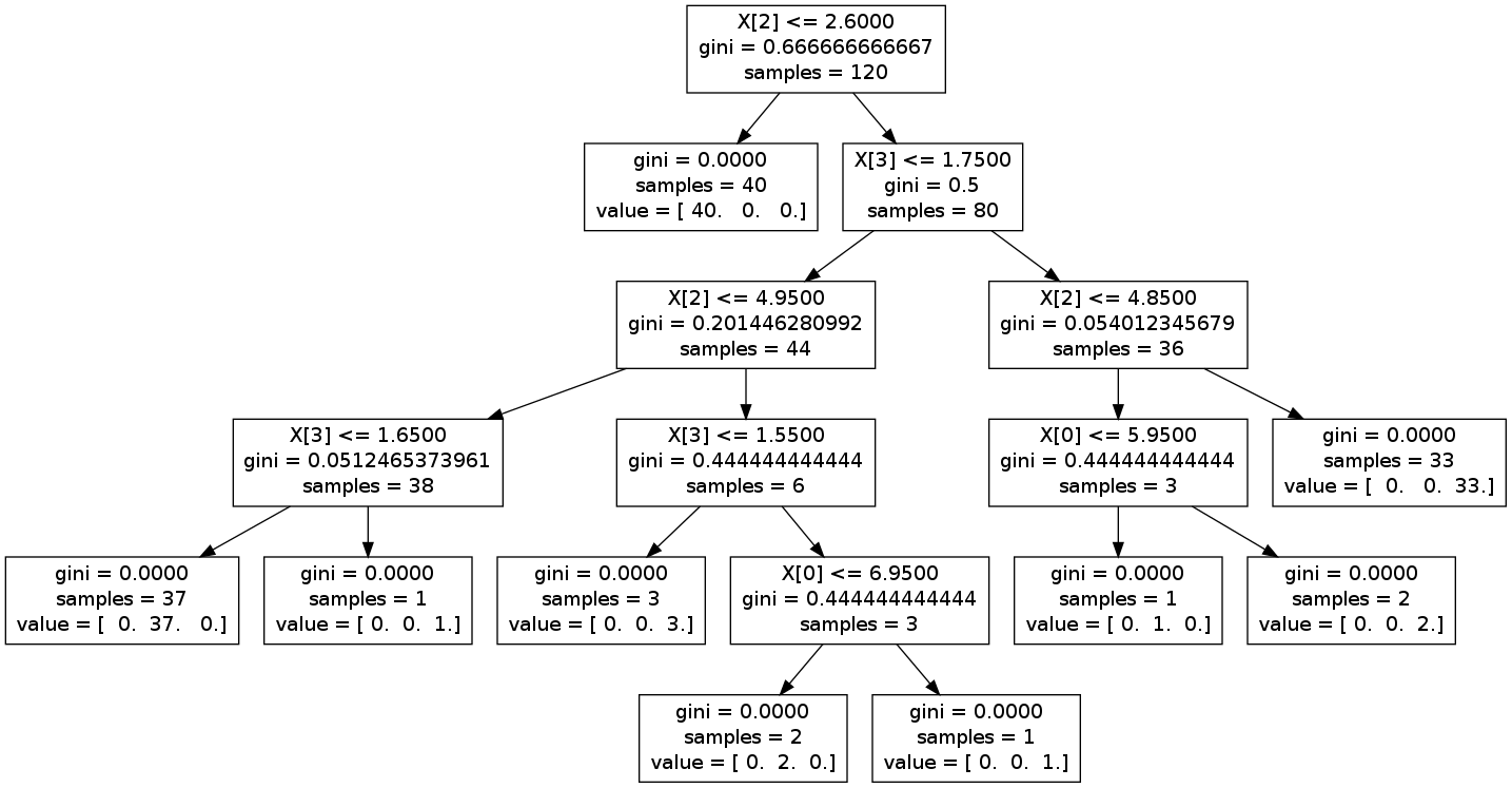
很明显，叶子节点具有value属性。iris有3个分类，故value有三个值，若第1个值比较大，认为是第1个分类；若第2个值比较大，认为是第2个分类；...。

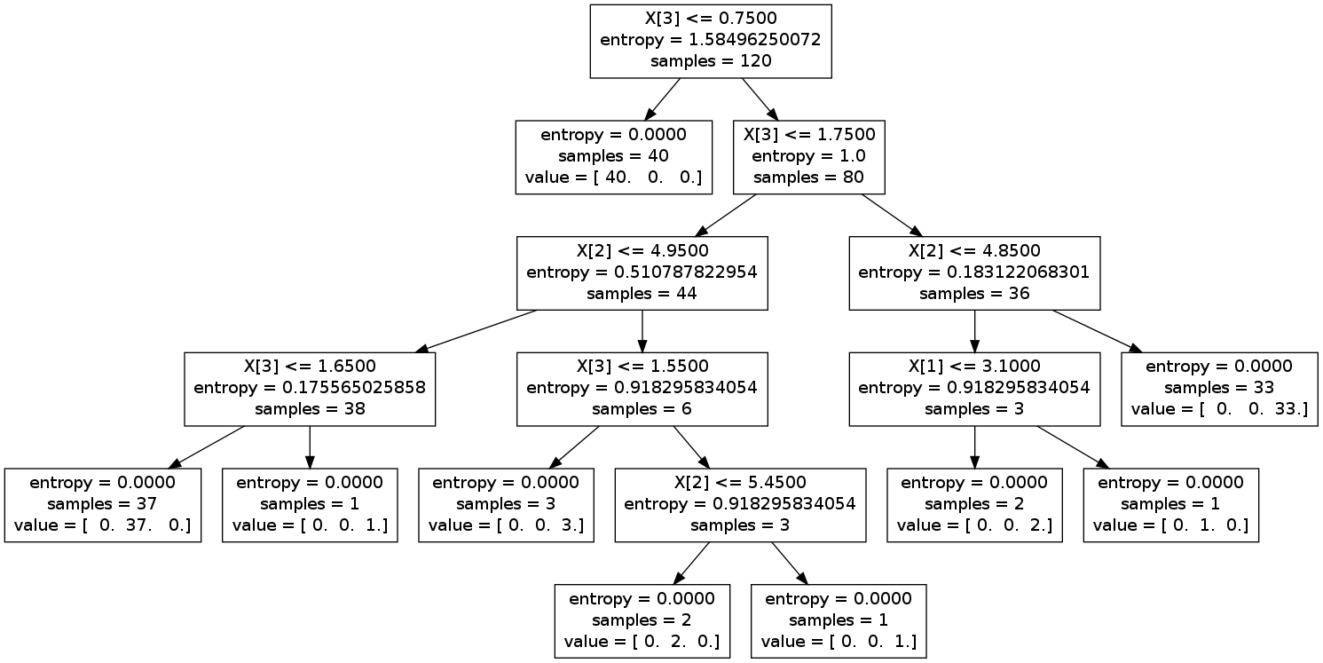
基于信息增益的决策树

Information Gain，信息增益。

>>> clf = DecisionTreeClassifier(criterion='entropy')
>>> clf2 = DecisionTreeClassifier(criterion='entropy')
>>> clf2.fit(train_data, train_target)
DecisionTreeClassifier(criterion='entropy', max_depth=None, max_features=None,
            max_leaf_nodes=None, min_samples_leaf=1, min_samples_split=2,
            min_weight_fraction_leaf=0.0, random_state=None,
            splitter='best')
>>> predict_target = clf2.predict(test_data)
>>> sum(predict_target == test_target)
30
>>> with open("iris2.dot", 'w') as out:
...     out = export_graphviz(clf2, out_file=out)

上图：

参考

http://scikit-learn.org/stable/modules/tree.html#tree

http://scikit-learn.org/stable/modules/generated/sklearn.tree.DecisionTreeClassifier.html

http://scikit-learn.org/stable/modules/generated/sklearn.tree.export_graphviz.html

Visualizing a decision tree ( example from scikit-learn)

使用决策树处理iris数据集

构造数据集

基于gini不纯度的决策树

基于信息增益的决策树

参考